Background
This short write up is in pursuit of a personal goal to put more of my work and thoughts to paper. I’m sure the topic will still be useful to others, but it’s not yet fully developed. It’s a sketch of a work in progress.
Last August, I took the fast.ai Practical Deep Learning for Coders online course (and worked through
the accompanying book). The course taught the fundamentals of deep learning using the fastai Python
library, which offers a higher-level API (and a vast range of useful features and tools) for
PyTorch. The course (and book) followed a “top-down” approach: learn how to effectively apply the
models first, and then go back and learn the more foundational concepts, math, etc., in greater
detail.
After spending several months using fastai for a number of tasks (including the Kaggle Cassava Leaf
Disease Classification competition, the numer.ai tournament, and a turtle classifier), I decided I
wanted to “pull back the curtain” and start to learn how to use PyTorch. The numer.ai tournament
seemed like an excellent opportunity to do so. The tournament data come in a very “clean” and
ready-to-use format, so grappling with the data doesn’t have to be a huge part of the modeling
process. The dataset is big enough for deep learning but not so huge that the models can’t be run
locally. And I already have a working fast.ai model up and running, and I know it’s running PyTorch
under the hood, so I know that it will work!
One quick note: trying to learn PyTorch is inspired by a desire to learn more; not by any serious
perceived weaknesses in fastai. Many fastai users and community members, such as Zachary Mueller
(see the excellent walk with fastai project) have shown that fastai is extremely flexible and
extensible. That said:
- Implementations of new methods often appear first as PyTorch models. Using them directly is easier
to me than translating them to a
fastaicontext. fastaisometimes hides so many details that I find it hard to determine what, exactly, my models are doing. For example, it took me a while to discover that thefastaitabular model I was using for the Numerai tournament was implementing batchnorm and dropout layers. The architecture of the model was, at least initially, opaque to me.- While
fastaiallows plenty of flexibility, it isn’t necessarily built for it. I often need to do quite a bit of research to figure out how to tweak my training loop in a way that would be trivial in a direct PyTorch implementation. - Some of the other learning resources I’ve been using, such as the excellent Dive into Deep
Learning book, use PyTorch. Rather than translating their code into
fastai, I would prefer to learn PyTorch directly.
In this post, I will first briefly show the fastai model I was previously using, and then introduce
a (simpler) model written in PyTorch. I will conclude with some reflections on the process.
Problem Setting
I won’t go into much detail about the Numerai tournament itself – the interested reader can learn more about it here. This isn’t intended as an introduction to the tournament and I’m not reproducing my whole data preparation and processing pipeline. That said, it should be very straightforward to apply the code here to data obtained from the tournament.
The features are all numeric and all take on values of 0, 0.25, 0.5, 0.75, or 1. The targets can take the same values. Numerai competitors have tested and discussed the impact of treating the targets as categorical rather than as numeric responses and have generally found that regression approaches work better than classification approaches. So we will treat this as a regression problem with numeric features and targets. The criterion we are trying to optimize is the Spearman’s rank correlation coefficient. That is, we want to be able to predict the order of the responses as accurately as possible. Most users approximate this by directly optimizing mean squared error (MSE); we will do the same.
An obvious question at this phase is: given a large number of observations but a small number of targets (recall: all targets take values of 0, 0.25, 0.5, 0.75, or 1), how exactly are we supposed to create a meaningful ordering? Well, there are a couple of answers to that. First and foremost: we’re only aiming for a rough ordering. If we could just make sure all of the “0” targets were predicted lower than all of the “1” targets, we’d be off to a great start! In general, in this problem, there is a lot of “noise” and very little “signal.” We’re not going to be able to precisely order all of the observations, so having only a few targets to work with doesn’t hurt as much as it may seem.
Second, it’s possible to obtain reasonably high Spearman correlation values when “blocks” of predictions are correctly ordered but when the observations within those blocks are completely shuffled. The figure below shows the results of a simulation wherein 5000 observations were divided into five targets roughly in proportion to those in the Numerai tournament. “Predictions” were generated such that all of the predictions in the lowest category were lower than all of the predictions in the next category for all categories. For example, any prediction in category 0.25 was guaranteed to be lower than any prediction in category 0.5. Within each category, however, the predictions were shuffled. This experiment was repeated 5000 times. The average Spearman correlation coefficient was 0.859 (the highest possible is 1).
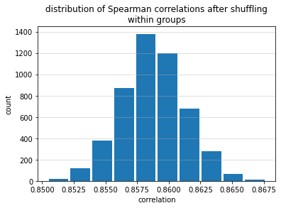
Figure 1: Even when predictions were shuffled within “blocks,” high Spearman correlation coefficients were obtained when those blocks were placed in order.
So even when large “blocks” of predictions were shuffled internally, as long as those “blocks” were ordered correctly relative to each other, the Spearman correlation coefficients remained high.
Original fastai model
My original fastai implementation does not differ appreciably from the implementation detailed in
the official fastai Tabular Training tutorial. The components are, briefly:
Data Setup
First, we use the TabularPandas helper to load the data and to generate our DataLoaders. DataLoaders
provide a convenient wrapper around the training and validation data and facilitate passing batches
of data to the model during the training loop.
Our data (including training and validation examples) exist in a Pandas DataFrame called
training_data. We have defined indices train_idx and val_idx corresponding to the training and
validation examples.
splits = (list(train_idx), list(val_idx))
data = TabularPandas(training_data, cat_names=None,
                    cont_names=list(feature_cols.values),
                    y_names=target_cols, splits = splits)

dls = data.dataloaders(bs = 2048)
Model Setup
We will use a fastai tabular_learner without much modification and without adjusting many of the
possible options. As noted above, we’re using the MSE loss function. fastai also lets us directly
specify that we want to see the Spearman correlation coefficient as a “metric.” It’s not used in the
optimization process, but we get to see the change in the Spearman correlation coefficient after
each epoch.
learn = tabular_learner(dls, layers=[200,200],
                        loss_func=MSELossFlat(),
                        metrics = [SpearmanCorrCoef()])
Training Loop
fastai handles the training loop for us – we don’t need to write it out manually. Here we say to
train the model for three epochs and to apply a weight decay (l2 penalty) of 0.1.
learn.fit_one_cycle(3, wd = 0.1)
Summary
Without going into too much detail – this is, after all, supposed to be a post about PyTorch, which I’ve scarcely mentioned so far – I want to highlight some of the key features and shortcomings of this approach:
- It’s concise: we’ve created a suitable data iterator, defined the model, and run through the training loop in only a few lines of code. The training loop in particular took only one line!
- A lot of detail is hidden. We rely on “sane defaults” to a very high degree. What is the model architecture? Which optimizer is used? How will information be presented to us throughout the training loop?
- It does readily expose some of the key hyperparameters we’ll likely wish to experiment with, such as weight decay and the number and size of layers. Ultimately, once we have a better understanding of the architecture, it’s also not too difficult to modify hyperparameters associated with dropout and batchnorm.
In short, this method gets you from a blank screen to a trainable deep learning model with some easily-accessible hyperparameters to optimize about as quickly as one could ask for, but it keeps a lot of the details hidden.
A Simple PyTorch Model
In an effort to learn some basic PyTorch, I set out to develop a very simple working model. It doesn’t have all of the bells and whistles of the fastai model – no batchnorm, no dropout, no weight decay – but it works and it is generally easy to understand what the model is doing. This provides a good foundation for further experimentation with more complex architectures.
Data Setup
A common theme throughout this section is that “It takes a bit more code to do ____ in PyTorch than
in fastai. Setting up the data is no exception. I mostly followed this guide for setting up the data
for use by the PyTorch model.
The biggest additional step is that we must define a
custom class inheriting from the PyTorch DataSet class. The class must define:
__len__(): a method for finding the length of the dataset; and__getitem__(): a method for returning an item from the dataset given an index.
I wrote the NumerData class for this purpose as shown below. Note that the data argument refers to
the whole training dataset; feature_cols is a list of the feature column names; and target_cols is a
named list of the target column names.
class NumerData(Dataset):
    def __init__(self, data, feature_cols, target_cols):
        self.data = data
        self.features = data[feature_cols].copy().values.astype(np.float32)
        self.targets = data[target_cols].copy().values.astype(np.float32)
        self.eras = data.era.copy().values

    def __len__(self):
        return(len(self.data))

    def __getitem__(self, idx):
        if torch.is_tensor(idx):
            idx = idx.tolist()

        return self.features[idx], self.targets[idx], self.eras[idx]
The dataset ended up being the biggest performance bottleneck for me, at least at first. I had
initially put off some amount of the processing to the __getitem__() method, which meant that every
time the DataLoader needed to return a new batch of data, it needed to do a lot more indexing and
processing than it should have. A couple of examples:
- I explicitly included type conversions (to tensors) in the
__getitem__()method. This was unnecessary as theDataLoaderhandles this by default. It also took time. - I made the
DataLoaderpull the features and targets from the full dataset each time instead of storing them as separate objects. That is, instead of justreturn self.features[idx], I first definedself.features = data[feature_cols]. This should be handled in the__init__()method, not each time__getitem__()is called.
Note that the NumerData class currently does not define any data. We need to instantiate an object of
type NumerData with some data in order to use it. We will define separate ~DataSet~s for the
training and validation data.
train_ds = NumerData(training_data.iloc[train_idx],
                     feature_cols, target_cols)

val_ds = NumerData(training_data.iloc[val_idx],
                     feature_cols, target_cols)
With these defined, we can use use the PyTorch DataLoader to handle iteration through the ~DataSet~s
in batches. Again, we instantiate separate ~DataLoader~s for our train and validation sets:
train_dl = DataLoader(train_ds, batch_size = 2048, shuffle=False, num_workers=0)
val_dl = DataLoader(val_ds, batch_size = len(val_ds), shuffle=False)
Now our data are ready to go and we can define the model.
The Model
The model has a few separate components – a fact that is easy to miss when working with
fastai. We need to define:
- The model architecture itself
- The loss function (or criterion)
- The optimizer
Furthermore, when defining the model, we need to be (just a little bit) mindful of the dimension of
our inputs (another thing fastai takes care of automatically). Ultimately, none of this is
particularly onerous:
n_feat = len(feature_cols)
net = nn.Sequential(nn.Linear(n_feat, 256),
                    nn.ReLU(),
                    nn.Linear(256, 1))

criterion = nn.MSELoss()
optim = torch.optim.Adam(params = net.parameters())
The model we have defined is a simple multilayer perceptron (MLP). Our input batch is passed to a
linear layer with 256 “neurons.” The output of this layer is passed to the ReLU(), or rectified
linear unit, layer. The output of this layer is passed to another linear layer, which produces the
one-dimensional output.
As noted above, we use MSE as our loss function. We use the Adam optimizer; details on this
optimizer can be found here.
The Training Loop
The training loop represents the part of the implementation where fastai provides the most help. In
fastai, the whole process is largely automatic. We called learn.fit_one_cycle(), specified the number
of epochs, and let the model run. But a lot is happening behind the scenes, and we need to write
that logic manually in PyTorch.
We will write a method to train a single epoch. We can then put this in a loop to train multiple epochs if needed.
def train(epoch, model):
    device = torch.device("cuda:0" if torch.cuda.is_available() else "cpu")
    model = model.to(device)

    # set up tqdm bar
    pbar = tqdm(enumerate(BackgroundGenerator(train_dl)),
                total=len(train_dl), position=0, leave=False)

    for batch_idx, (data, target, era) in pbar:
        data, target = data.to(device), target.to(device)

        # reset gradients
        optim.zero_grad()

        # forward pass
        out = model(data)

        #compute loss
        loss = criterion(out, target)

        #backpropagation
        loss.backward()

        #update the parameters
        optim.step()

        if batch_idx % 100 == 0:
            print(f'Train Epoch/Batch: {epoch}/{batch_idx}\tTraining Loss: {loss.item():.4f}')
In this method, we:
- Identify whether we have a GPU available for training and, if so, pass the model to the GPU.
- Using the
tqdmpackage, set up a progress bar for tracking model progress. - For each batch in the
DataLoader:- Send the features/targets to the appropriate device (GPU if available)
- Reset the gradients
- Compute the forward pass: pass the batch through the model and compute the outputs for each observation in the batch
- Compute the loss
- Back-propagate (compute the gradient of the loss function with respect to the weights)
- Update the weights
- Occasionally print the training loss
We can define a similar method for evaluating our model performance on the validation set (without
updating model weights). Suppose we’ve defined a function called era_spearman to calculate the
average Spearman correlation coefficient across Numerai tournament eras in the validation data. Then
we can define a validation method as:
def test(model):
    device = torch.device("cuda:0" if torch.cuda.is_available() else "cpu")

    test_loss = 0
    with torch.no_grad():
        for data, target, era in val_dl:
            data, target = data.to(device), target.to(device)

            out = model(data)
            test_loss += criterion(out, target).item() # sum up batch loss
            val_corr = era_spearman(preds = out.cpu().numpy().squeeze(),
                                    targs = target.cpu().numpy().squeeze(),
                                    eras = era)

        #test_loss /= len(val_dl.dataset)
        print(f'Test Loss: {test_loss:.4f}, Test Correlation: {val_corr:.4f}')
This follows much of the same logic as the training method, with some key exceptions:
- Everything happens under the
torch.no_grad()context handler. Why? We’re only using the validation data to assess the performance of our model; we don’t want to compute any gradients and we certainly do not want to use these data to update our model weights. - We make sure to calculate the metric we’re really interested in (the Spearman correlation). This is useful to check in case the loss function (MSE) does not actually improve the Spearman correlation.
- In this particular case, I did not divide the validation data into batches (put differently, the batch size is the length of the validation set). It certainly could have been divided into batches, though, and doing so may be necessary with larger datasets or in the face of significant memory constraints.
Train the Model
We can finally train the model! This part is a simple for loop.
for epoch in range(6):
    train(epoch, net)
    test(net)
Summary
I wrote a lot more code to implement a comparatively-simple PyTorch model than to implement the
fastai model. The PyTorch model forces us to better understand the structure of the model and the
logic of the training loop, though it likely takes more time and more finessing to obtain an
efficiently-performing model with decent results. The fastai model, on the other hand, is very quick
to implement but does not expose as many of the details. It is relatively quick and easy to get a
model running and returning decent results, but it can take a bit more work to understand the
structure of the model and of the training loop.
I’ll be writing more – and more complicated – PyTorch models in the future. I hope to add in some
of the additional features included in the fastai tabular implementation, such as dropout layers. I
also want to experiment further with regularization – L2 penalization is very easy to use in
PyTorch, but I’ve found L1 penalization to work far better for regression models in the Numerai
tournament and I want to see if that distinction also holds true for regression models.