Example 1

This is example 1.6 on page 21 of Introduction to Linear Optimization (Bertsimas and Tsitsiklis 1997, 27). Our aim is to minimize the function \(-x_1-x_2\) subject to the following constraints:

\[\begin{align*} x_1+2x_2 \leq 3 \\ 2x_1+x_2 \leq 3 \\ x_1,\ x_2 \geq 0 \end{align*}\]

Visualizing the feasible set

First, we want to see what sorts of values the feasible set can take on. We begin by defining our objective function for later use:

#Objective function
obj.fun=function(x) -x[1] - x[2]

Next, we plot our constraints and determine which values of \(x_1\) and \(x_2\) fall into the feasible set. Note that both \(x_1\) and \(x_2\) are bounded above by \(3\) and below by \(0\) by the problem definition, so we restrict our attention to \(x = (x_1,x_2) \in [0,3] \times [0,3]\).

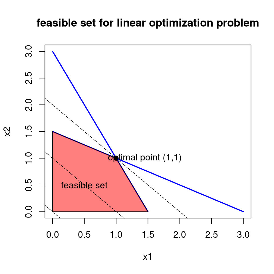
We will place \(x_1 \text{ and } x_2\) on the x and y axes, respectively. We draw lines between the intercepts of the constraints by noting that \(x_1+2x_2=3\) at points on the line connecting \((0,1.5)\) and \((3,0)\). Likewise, we represent \(2x_1+x_2=3\) by points on the line connecting \((1.5,0)\) and \((0,3)\). Since \(x_1 \geq 0\) and \(x_2 \geq 0\), the area between these lines and the axes represents the feasible set.

# setting up vertices for shading with polygon
x.vert=c(0,1.5,1,0)
y.vert = c(0,0,1,1.5)

plot(1,xlim=c(0,3),ylim=c(0,3),xlab="x1",ylab="x2",lty=2,lwd=1.5,
   main="feasible set for linear optimization problem")
lines(c(0,3),c(1.5,0),lwd=2,col="blue")
lines(c(0,1.5),c(3,0),lwd=2,col="blue")
polygon(x.vert,y.vert,col=rgb(1,0,0,0.5))
abline(0,-1,lty=4)
abline(1,-1,lty=4)
abline(2,-1,lty=4)
points(1,1,pch=19)
text(1.45,1,"optimal point (1,1)")
text(0.5,0.5,"feasible set")

The red shaded region represents the feasible set. The blue lines represent the two constraint inequalities.

Note that we want to minimize \(-x_1-x_2\) which is equivalent to maximizing \(x_1+x_2\) within the given constraints. It is clear from the plot that the point \((1,1)\) maximizes \(x_1+x_2\) within the feasible set. Putting this into the original, we obtain \(-x_1-x_2 = -1-1 = -2\), so \(-2\) is the minimum.

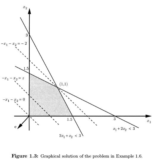
Plotting this was not entirely straightforward. The textbook image is easier to read:

textbook image

In particular, I liked that the lines extended past the axes, and I thought the lines were well-labeled. That was fairly difficult for me to do in the base R plotting system. I’m sure these things can be done in the basic R plotting package. I will tackle that in a future post.

Optimizing with R’s built-in package

We conclude by quickly verifying the result we obtained through graphing by using R’s constrOptim() function.

Note that the gradient is \(\nabla f(x)= \begin{pmatrix}-1\\-1\end{pmatrix}\). We choose a starting value of \(\begin{pmatrix}0.1\\0.1\end{pmatrix}\) which is in the feasible set. In the constrOptim function, the constraints are defined such that ui %*% theta - ci >= 0. To put the constraints in this form, we define \(\textbf{ui}=\begin{pmatrix}-2 & -1\\ -1 & -2\end{pmatrix}\) and \(\textbf{ci}=\begin{pmatrix}-3\\-3\end{pmatrix}\). We these arguments, we use the constrOptim() function like so:

grad=function(x1,x2) c(-1,-1)
minim=constrOptim(theta=c(.01,.01),f=obj.fun,grad=grad,
            ui=rbind(-1*c(2,1),-1*c(1,2)),ci=-1*c(3,3))

And we obtain the following values for the minimizer and minimum.

## $par
## [1] 1 1

## $value
## [1] -2

This corresponds to what we obtained by plotting the constraints. My next post on linear optimization will look at another example and will attempt to generate a more informative plot.

References

Bertsimas, Dimitris, and John N. Tsitsiklis. 1997. Introduction to Linear Optimization. Third printing edition. Belmont, Mass: Athena Scientific.