Installing OpenBUGS

First of all, I am running Arch linux with kernel version x86_64 Linux 4.14.13-1-ARCH. I was not able to find any one-step installation package, so I followed the instructions on the OpenBUGS site. The OpenBUGS site instructs the user to do the following:

Download and Unpack the package

tar zxvf OpenBUGS-3.2.3.tar.gz
cd OpenBUGS-3.2.3

Compile and Install

./configure
make
sudo make install

And, if your system has all of the necessary dependencies, that’s it! My system, however, did not have the necessary dependencies – there are some 32-bit C development packages required for installation. I installed the following packages in response to various error messages in the installation process: lib32-glibc, lib32-gcc-libs, gcc6-libs, gcc6. I’m not certain that all of those are strictly necessary, and I can’t guarantee others won’t be required: read the installation logs/error messages for details. After installing those packages, the rest of the installation went smoothly.

Making OpenBUGS talk to R

I use R daily, so for me, it made sense to set up OpenBUGS to run within my existing R analysis/programming workflow. To that end, we install two packages, R2OpenBUGS and coda. I will explain what they do later. As with any other packages, install these in an R session with install.packages(c("R2OpenBUGS","coda"))"

Loading required packages

As noted earlier, we require a couple of packages to carry out the analysis. They can be loaded as follows:

library("R2OpenBUGS")
library("coda")
library("lattice")

Defining our model

We define our model as an R function. We will never actually call this function, but this format allows the R2OpenBUGS package to properly invoke the OpenBUGS system. Note that the code within the function is taken directly from Carlin and Louis’s book. Note as well that, when defining variables in our model definition, we must use <-; using an equals sign = will return an error. The tilde ~ means that a parameter follows a particular distribution.

Per the bugs (from the R2OpenBUGS package) function help documentation (viewed with ?bugs), the model has to be saved as a .txt file. We save it to the /tmp directory using the write.model from the the R2OpenBUGS package.

model=function(){
  prec.ybar<-n/sigma2
  prec.theta<-1/tau2
  ybar~dnorm(theta,prec.ybar)
  theta~dnorm(mu, prec.theta)
}

# write the model to a .txt file, save to /tmp
model.file=file.path(tempdir(),"model.txt")
write.model(model,model.file)

Defining our data and parameters of interest

In this case, we only have one data point. We are treating this as a univariate problem, so we supply values for \(\mu\), \(\sigma^2\), and \(\tau^2\). The only parameter we want to perform inference on, in this case, is \(\theta\), so we must indicate this before running our BUGS process as well.

data=list(ybar=6,mu=2,sigma2=1,tau2=1,n=1)

# parameter
params=c("theta")

Defining inital values

For the algorithm to work, we must supply plausible starting values for our parameters of interest. In this case, we are only interested in \(\theta\), so only need to supply a starting value for \(\theta\). As with the model, we also define the inital values as a function. Once again, R will not call this function, but defining it this way allows OpenBUGS to access it.

inits=function() {list(theta=0)} 

Inference with BUGS

Now we call the bugs() function to run OpenBUGS from R. We pass the data, inital values, parameters, and model file as defined above.

out=bugs(data,inits,params,model.file,n.iter=10000) 

From this, we can obtain (among other things) the mean and standard deviation of our parameter.

out$mean["theta"]

## $theta
## [1] 3.99604

out$sd["theta"]

## $theta
## [1] 0.7107001

Coda

Recall that, earlier, we installed and loaded the package coda. This package provides a set of tools for summarizing and visualizing results from Markov-chain Monte Carlo simulation experiments. It also has a suite of diagnostic tools, but we will not be focusing on those capabilities in this post. We will use the coda package to plot our distribution.

To use coda, we need to make a slight adjustment to our call to bugs – we need to add codaPkg=TRUE to the function call. Once that is done, we can easily see the density of our distribution.

out=bugs(data,inits,params,model.file,codaPkg=TRUE, n.iter=10000)
coda.out=read.bugs(out)

## Abstracting deviance ... 5000 valid values
## Abstracting theta ... 5000 valid values
## Abstracting deviance ... 5000 valid values
## Abstracting theta ... 5000 valid values
## Abstracting deviance ... 5000 valid values
## Abstracting theta ... 5000 valid values

densityplot(coda.out)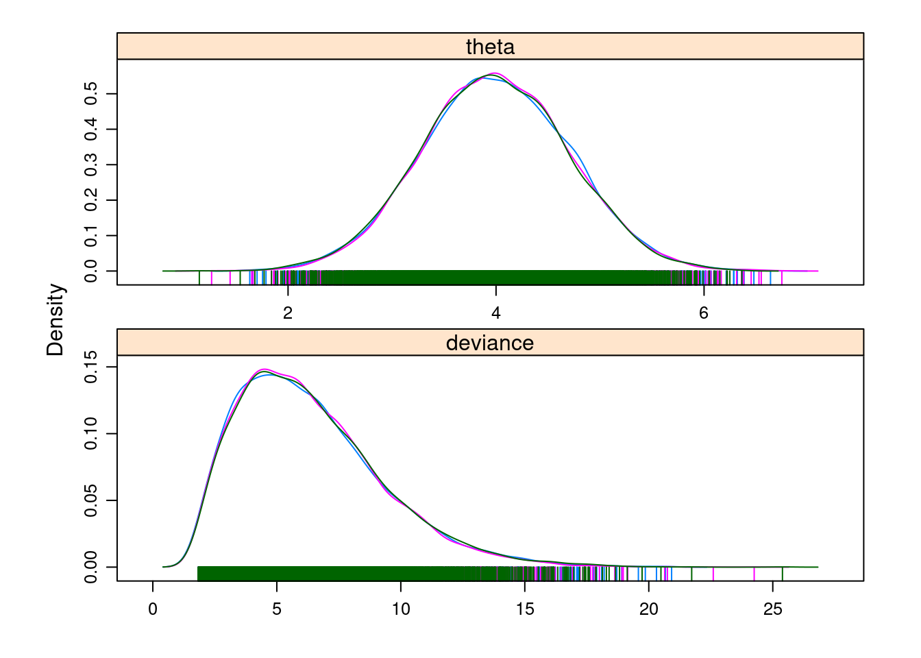

What we see resembles a normal density with a mean around 4. This makes sense given that the prior mean was 2 and the data sample mean was 6, and the variances of the two were the same.

Conclusion

This was a quick guide to get up and running with OpenBUGS and R on a Linux system. In future posts, we’ll delve into some more of the nuts and bolts of how to use OpenBUGS and how to interpret the results in light of general Bayesian data analysis principles and practices.