Introduction
This is a followup to a prior post on the same topic, where I used R’s base plotting system to visualize a linear programming provelm. I’m again looking at section 1.4 of Introduction to Linear Optimization. This time, we’ll consider Example 1.8 on page 23 (Bertsimas and Tsitsiklis 1997, 23). The optimization problem in this example is:
\[\begin{align*} -x_1+x_2 &\leq 1 \\ x_1 &\geq 0 \\ x_2 &\geq 0 \end{align*}\]
Some preliminary notes
- This time, instead of using the base R package, we’re going to plot the problem using the
ggplot2package (Wickham 2009). - This example is meant to illustrate that there may not be a unique optimal solution and that the feasible set will not necessarily be bounded. For example, given the cost function \(x_1+X_2\), which we can represent with the vector \(c=(1,1)\), the unique optimal solution is \(x=(0,0)\). However, given the cost function \(x_1\) \((c=(1,0))\), we have infinite possible solutions. Setting \(x_1\)=0, any choice of \(X_2 \leq 1\) will be an optimal solution; that is, our solution has the form \(x=(0,x2)\).
We can explore some of these possibilities with R’s optimization functions. We begin with the first example, with cost vector \(c=(1,1)\):
# Objective Function 1: x1+x2
obj.fun=function(x) x[1] + x[2]
# gradient
grad=function(x1,x2) c(1,1)
minim=constrOptim(theta=c(.01,.01),f=obj.fun,grad=grad,
                              ui=rbind(c(-1,1),c(1,0),c(0,1)),ci=c(-1,0,0))
The unique minimizer of this cost function is 0, 0 and the minimum is, as expected, 0.
But what happens when we try this in a case without a single optimal solution? Now we will try the second case discussed above. The code is largely the same, but we change our objective function.
# Objective Function 1: x1+x2
obj.fun=function(x) x[1] + 0
# gradient
grad=function(x1,x2) c(1,0)
minim=constrOptim(theta=c(.01,.01),f=obj.fun,grad=grad,
                              ui=rbind(c(-1,1),c(1,0),c(0,1)),ci=c(-1,0,0))
This returns 0, 0 as the minimizer and 0 as the minimum. In this case, \(X_2\) remained practically unchanged from the initial value. So the function worked for identifying an optimal solution, but it is important to be remember that this is not a general solution and \(x_2\) can take on any value in the feasible set.
Plotting the problem
Again, we are going to use ggplot2 to construct the plot this time. As in the first example, we will show \(x_1\) on the horizontal axis and \(x_2\) on the vertical. We follow this guide for some tips on how to plot functions with ggplot2.
Defining the function
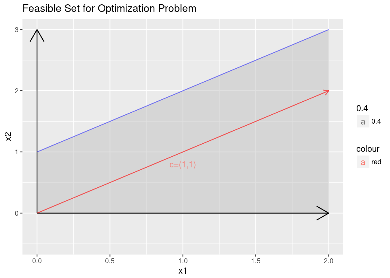
Let’s think of \(x_2\) as a function of \(X_1\) for the sake of this visualization problem. We can represent \(-x_1+x_2 \leq 1\) as \(x_2 \leq 1+x_1\). If we plot \(x_2=1+x_1\), everything under the curve will satisfy that constraint. To satisfy our other conditions, \(x_1\geq0\) and \(x_2 \geq 0\), we will simply consider the area above the horizontal axis and to the right of the vertical axis.
constraint=function(x1) 1+x1Plotting
We use the stat_function argument to plot our constraint line (recall: a function of x1) and to fill in the area beneath it, representing the feasible set. The red lines show possible solutions.
ggplot(data.frame(x=c(0, 2)), aes(x)) +
  stat_function(fun=constraint, geom="area",fill="gray76",alpha=0.5) +
  stat_function(fun=constraint, geom="line",col="blue",alpha=0.5) +
  geom_segment(mapping=aes(x=0,y=0,xend=2, yend=0), arrow=arrow(), size=0.5) +
  geom_segment(mapping=aes(x=0,y=x,xend=0, yend=3), arrow=arrow(), size=0.5) +
  ylab("x2") + xlab ("x1") +
  ggtitle("Feasible Set for Optimization Problem") +
  ylim(-0.5,3) +
  geom_segment(mapping=aes(x=0,y=0,xend=2, yend=2),
               arrow=arrow(length = unit(0.1,"inches")),
               size=0.5,col="red",alpha=0.4) +
  geom_text(aes(x=1,y=.8,label="c=(1,1)",col="red",alpha=0.4))
Looking at this can tell us a lot about our possible solutions. It is clear, for instance, that the unique minimum for the cost function \(x_1+x_2\) lies at \(x=0,0\): any other values of \(x_1\) or \(x_2\) in the feasible set will result in a larger cost. The line is plotted in red in the figure above. Similarly, if we consider \(x_1+0 \times x_2\), we can see that choosing \(x_1=0\) and any \(x_2\) value in the feasible set will return the (non-unique) minimum. For example, choosing \(x_1=0\) and \(x_2 = 2\) will give us \(0+0 \times 2=0\).
Bertsimas, Dimitris, and John N. Tsitsiklis. 1997. Introduction to Linear Optimization. Third printing edition. Belmont, Mass: Athena Scientific.
Wickham, Hadley. 2009. Ggplot2: Elegant Graphics for Data Analysis. Springer-Verlag New York. http://ggplot2.org.